 Cameron Davidson-Pilon
Part of our bioreactor project depends on the ability to track microbial population sizes. If you read our last blog article, you’ll know that we measure the population size by the amount of light scattering off the cells and hitting a photodiode. Therefore more light hitting the photodiode ⇒ more cells (up to a limit, but we can ignore that for now). However, this relationship is only proportional, and unless we calibrate our light readings against known cell densities, we don’t know the exact cell density. We’ll see that this isn’t a big deal later. But just know that we are working with optical density only.
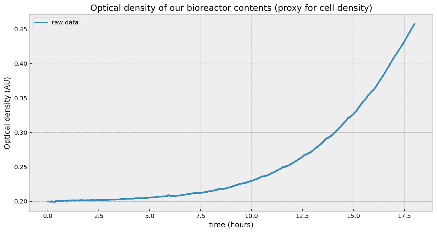
If the microbes are happy and healthy, they will be replicating, and our optical density will increase exponentially, that is,
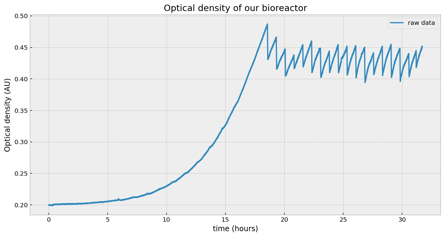
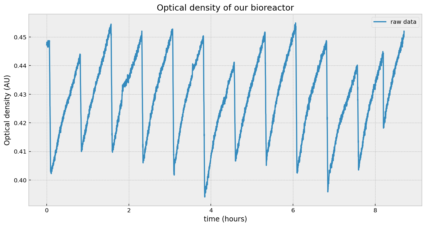
\[\text{OD}_t = \text{OD}_0 \exp{(r\cdot t)}\]And, after taking measurements, this is what we get:
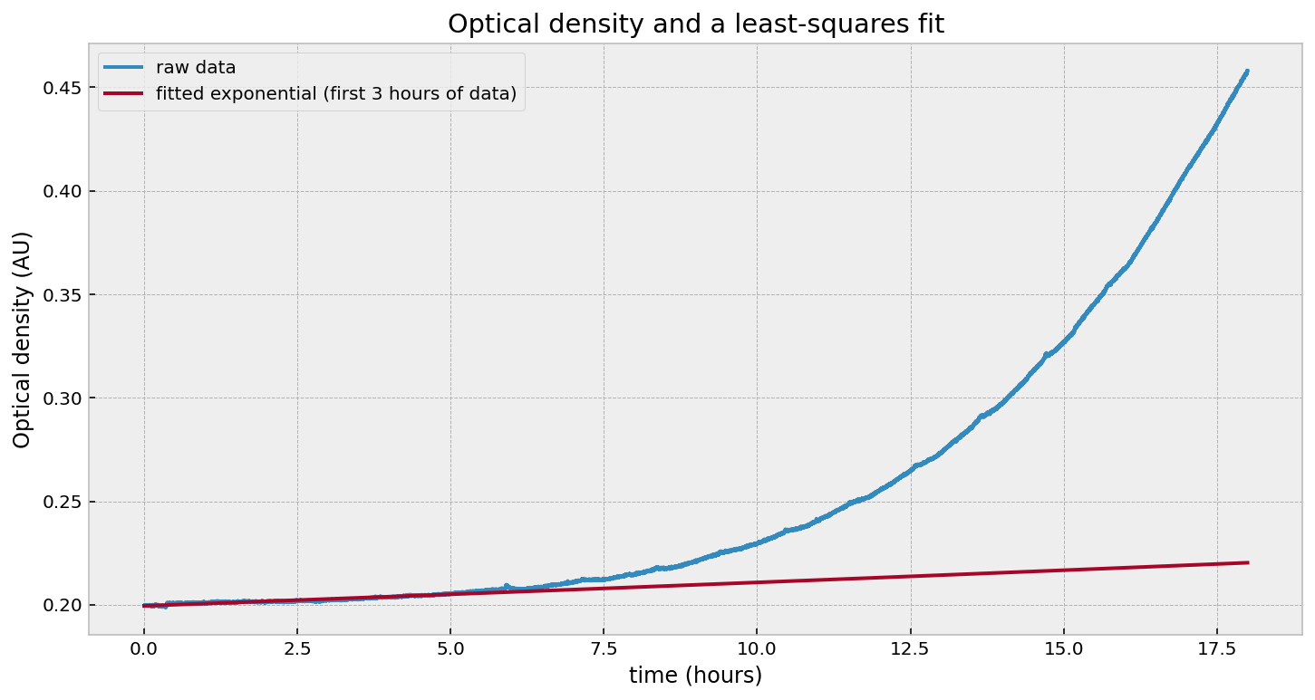
That looks exponential, right? Well, it is and it isn’t. Let’s first test an exponential by fitting this curve to an exponential model using least-squares:
from scipy.optimize import curve_fit

def exp_(x, A, rate):
    return A*np.exp(rate * x)

results, _ = curve_fit(exp_, x, y, p0=[0.2, .01])
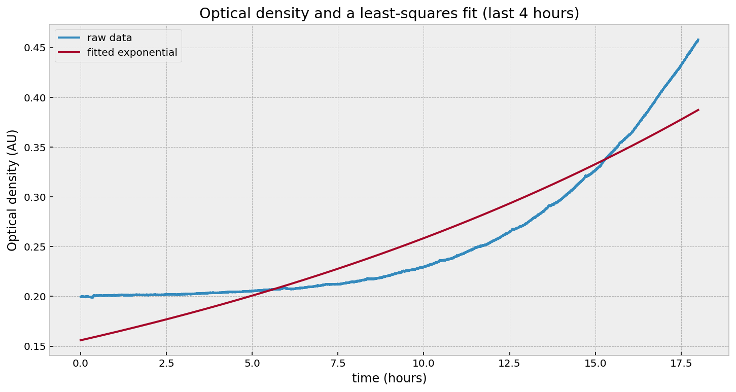
Wait - what happened? Why is the fit so poor? Let’s try just fitting to the last few hours:
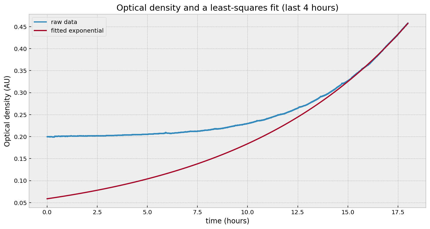
That looks good in the last few hours, but fails everywhere else. Likewise, if we fit to the beginning:
Yuck. What’s going on? The problem is that our growth rate parameter is not constant, so there is no good single value of $r$. Our model should in fact be:
\[\text{OD}_t = \text{OD}_0 \exp{(r_t\cdot t)}\]Note the subscript $t$ on the growth rate, $r$. This makes biological sense. Individuals cells, due to variation, will start to reproduce at different times, leading to an increasing population growth rate. Eventually, the growth rate will level off as all cells are actively reproducing (and, given a long enough time, the growth rate will creep up due to evolution). Now that we have a better mathematical model of our population, how can we estimate $r_t$?
To solve this, we will use a Kalman Filter. A Kalman Filter is an algorithm used for estimating a time-varying process that contains an internal dynamical system. Let’s break that down: estimating is the act of taking in noisy measurements and producing a more accurate result; time-varying process is an object that changes over time (in our case: both optical density and growth rate change over time); dynamical system is a model to describe the relationship between our variables: optical density and growth rate. I’d love to go into detail about how a Kalman Filter works, but for a computation-first-mathematics-second resource, I suggest the book I used: Kalman and Bayesian Filters in Python.
To start, we’ll write down the variables we wish to estimate (these are called our state variables):
\[\text{OD}_t\] \[r_t\]We can also write down a mathematical model of how these are related to each other and their previous values:
\[\begin{align*} \text{OD}_t &= \text{OD}_{t-1}\exp{(r_{t-1} \cdot \Delta t)}\\ r_{t} &= r_{t-1} \end{align*}\]That is, the next optical density is the previous optical density, multiplied by some growth rate. The growth rate is the same as the previous growth rate. Wait - the growth rate is the same as the previous growth rate? I thought we wanted to model a time-varying growth rate? We do, and these equations aren’t complete. There’s an additional noise term:
\[\begin{align*} \text{OD}_t &= \text{OD}_{t-1}\exp{(r_{t-1} \cdot \Delta t)} + \text{noise}\\ r_{t} &= r_{t-1} + \text{noise} \end{align*}\]We usually don’t write the noise terms in the dynamical system, but they are there. The noise terms will allow the rate term to evolve over time.
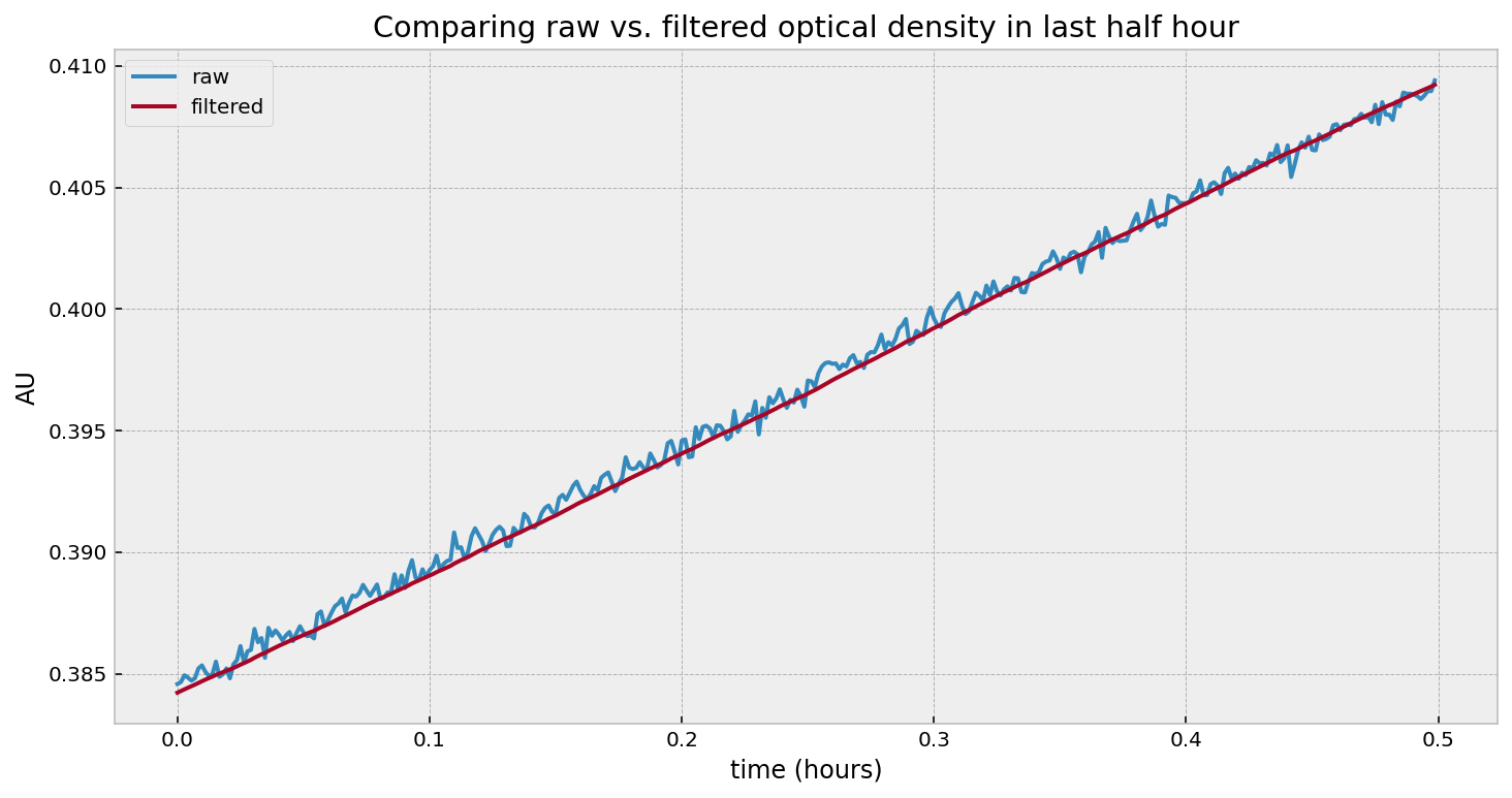
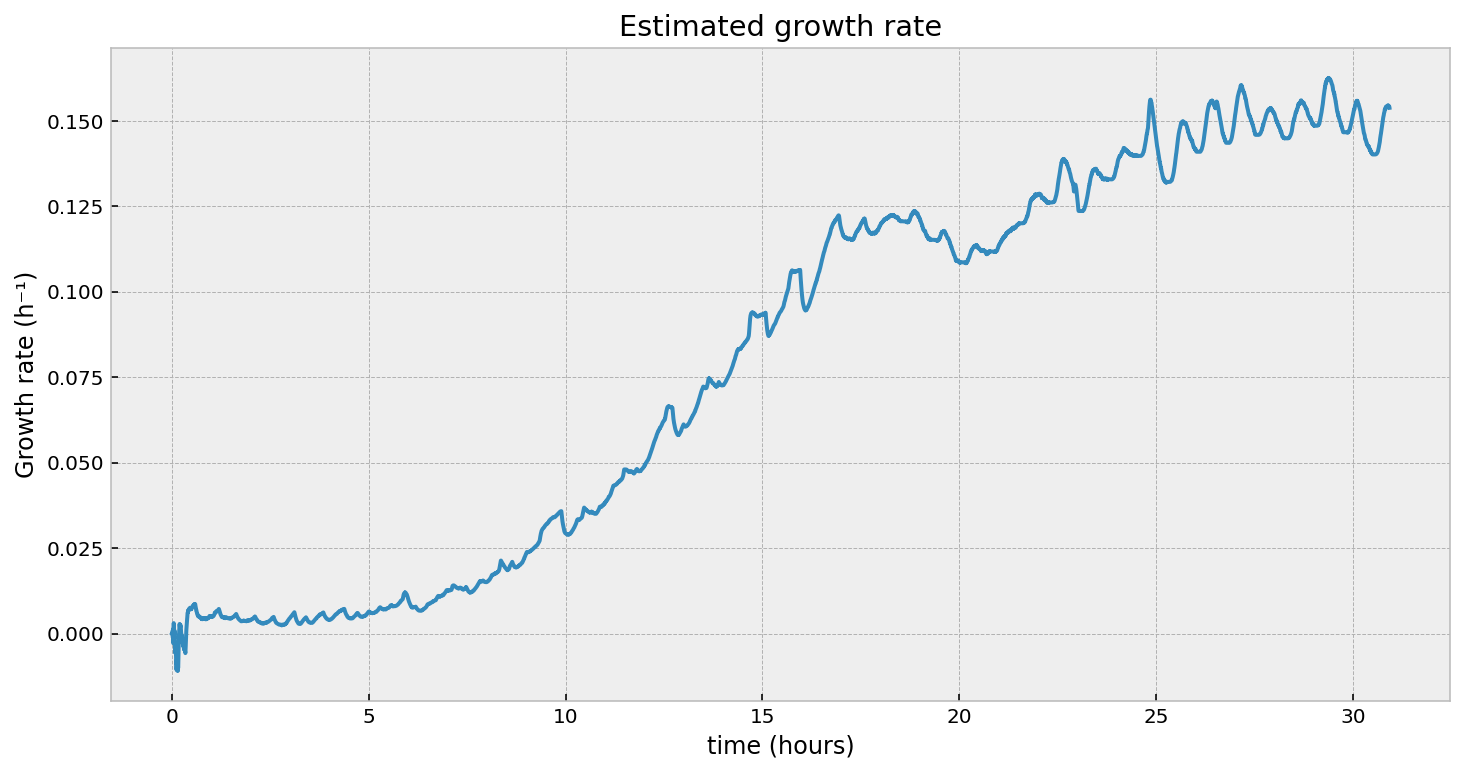
Without getting further into the math, we can test using a Kalman Filter on our problem above. At the end, we should have a “filtered” version of our optical density (think of it as smoothed - the noise has been eliminated), and a time-varying estimate of our growth rate.
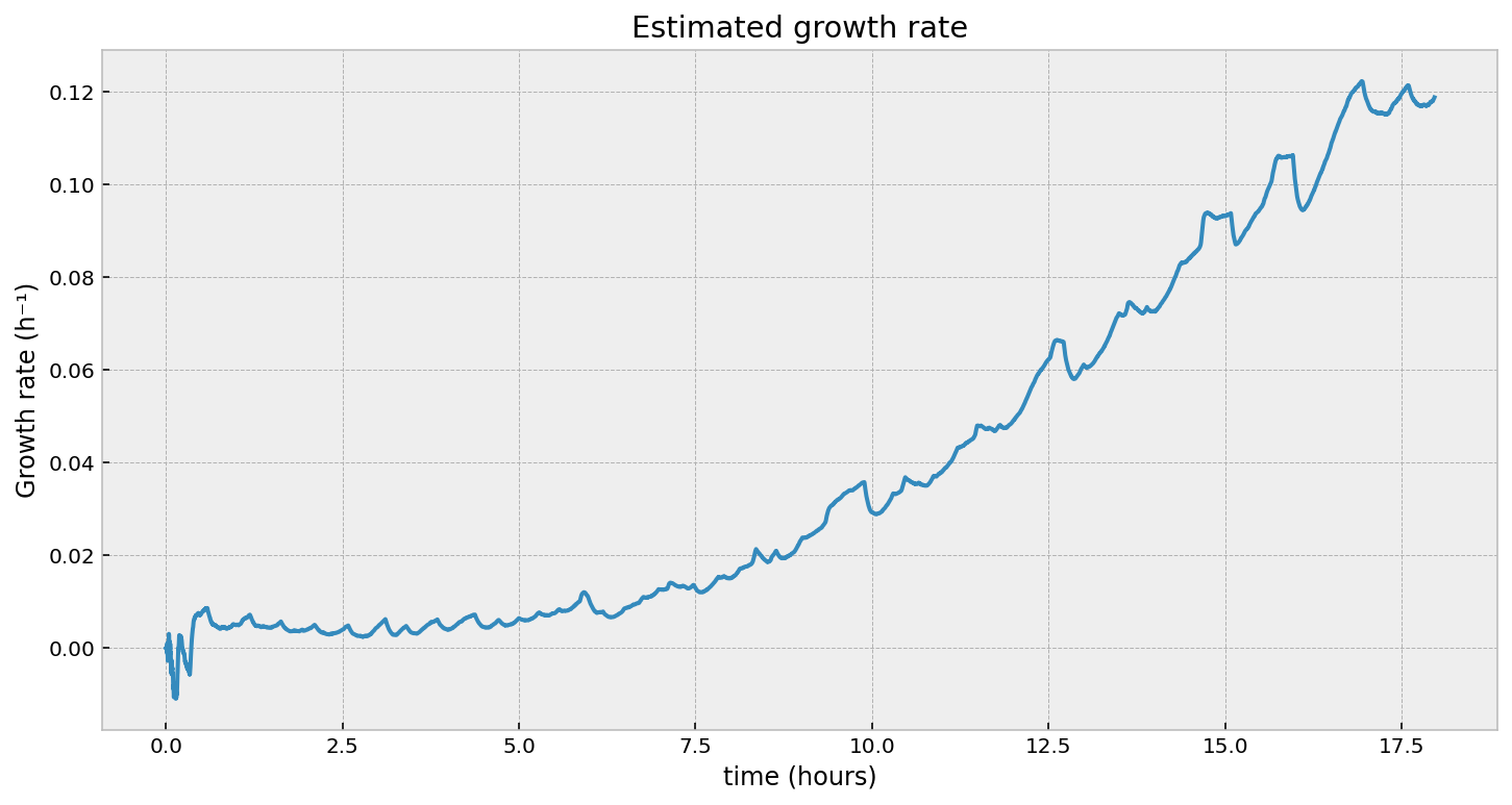
Looking at the second figure, the estimated growth rate, we can see that indeed the growth rate is increasing over time. It is always positive, which means the population will still be exponentially increasing at all times (as observed). However, we see some “noise” in it - what are those periodic bumps in the right of the graph? If we go back to the first figure in the article, we can see little blips in the optical density - our growth rate estimate is picking these up. It turns out, the room’s heating turning on is causing these bumps. It’s cool that we can pick these minor disturbances up.
This is great - we now have the following:
- A time-varying estimate of growth rate (as we expect biological populations to have a time-varying growth rate).
- The nature of the estimation also allows us to perform this in real time. That is, given a new OD measurement, we can pass it into our Kalman Filter and produce a new estimate of the growth rate at that time. This means we have immediate data for decision making. Compare this to the traditional “batch” process: take the past 30 minutes of data, run it through a curve-fitter, produce an estimate. You might say: well this works, too - if our 30 minute window is sliding, we can always produce an up-to-the-second growth rate estimate from the past 30 minute window. Here are some problems:
- Why 30 minutes? Why not 10 minutes, or 1 minute? There’s a bias-variance tradeoff to make here.
- If the growth rate is changing quickly, your window may be too long and you’ll miss the movements.
- What happens when there is a dilution event?
Dilution events
What is a dilution event? Well, the nature of exponential growth is that it will grow without bound. Obviously there is an upper limit based on the amount of nutrients, but we would like to keep our culture in a state of exponential growth. This requires is to periodically expel some liquid, and add in fresh media. This causes a reduction of the overall cell density, and therefore a reduction in the optical density too. You can see this in the figure below. The dips on the right-hand side is us removing some fraction of liquid and replacing it with fresh media. In fact, this is on a scheduale, and we perform this dilution every 45 minutes.
From the point-of-view of our Kalman Filter, it will get confused about these drops in OD: it would say “wowow lots of negative growth!” - but we know that’s not true. The growth rate shouldn’t vary over a dilution event - the change in OD is due to a physical process, not a biological one.
Luckily, Kalman Filters can be “hacked” to include external information. I’ve programmed just this (taking inspiration from this paper). Basically, during the dilution events, we increase the noise many fold, causing all the estimates to “freeze”, until the noise is back down when the dilution event ends.
What’s up with the oscillations on the right? Are those artifacts of our hack? Actually no, it’s a real phenomenon. Zooming in on the dilution events:
We can see that the growth rate is not constant between dilution events, and does vary up then down. Our Kalman Filter (for better or worse) picks this up.
Sensor fusion
Using a Kalman Filter allows us to combine multiple sensors into a single estimate. For example, in our bioreactor, we actually have multiple photodiodes placed at different angles. Different angles have different sensitivities. We would like some way to combine all these photodiode measurements together. Ideally, this new estimate should have a smaller variance than estimates provided from not combining measurements (spoiler alert: it does have smaller variance). The different sensors don’t even have to be the same type. Suppose I have a carbon dioxide sensor in the headspace. As the cells grow, they will produce more and more CO₂. If I have a model of how CO₂ is related to the growth rate, I can include this (possibly very noisy) measurement and get a more accurate growth rate estimate.
Modeling saturation
I mentioned above that the light scattering is proportional to cell density up to a limit. That limit is called the saturation point. Beyond this point, the relationship is no longer linear, but sub-linear. This is because there are so many cells that light that would previously have scattered into the photodiode is now being scattered away. There are atleast two solutions:
- Use angles that have a higher saturation point, like 90°. This comes at a cost of sensitivity though.
- Model the saturation in our dynamical system.
The latter might look like:
\[\begin{align*} C_t &= C_{t-1} \exp{(r_{t-1} \cdot \Delta t)}\\ \text{OD}_t &= f(\text{C}_{t-1}, \theta)\\ r_{t} &= r_{t-1} \end{align*}\]where $f$ is some linear function up until $\theta$, our saturation limit, and sub-linear beyond that, and $C_t$ is a (hidden) state of cell population. The $\theta$ can be estimated in the Kalman Filter, too. I haven’t implemented this yet, though!
Conclusion
To be honest, I have a love-hate relationship with Kalman filers. They enable some amazing inferences, like in our example above, that would otherwise be unreachable. However, they come with lots of parameters that need tuning. This has been a pain for me, as it’s not always clear how the model will change with respect to changing a parameter. The book I mentioned above, Kalman and Bayesian Filters in Python, has certainly helped with this, though.
Now that we have a good estimate time-varying growth rate, we monitor how the culture reacts to different environments. By controlling the environment, we can control the growth rate. So by surpressing the growth rate using the environment, we are introducing “headspace” for the microbes to evolve into. We’ll explore this next article.