Measuring cell density using a Secchi stick (and lots of math)

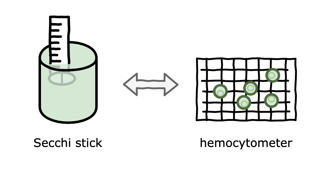
In liquid-state fermentation, like yeast, bacteria or algae cultures, one of the most important metrics is cell density, that is, how many cells there are per mL. This metric gives you an idea of where the cultures is in its lifecycle (see figure 1), and is obviously correlated to important outcomes like biomass.

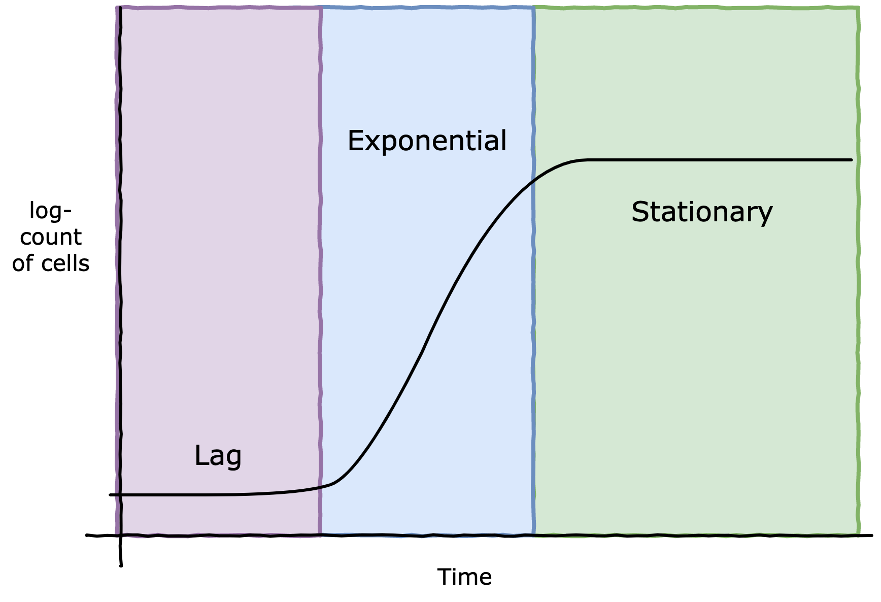Figure 1. Cell culture lifecycle - note the logarithmic scale

The traditional way to measure cell density is to use a microscope and a hemocytometer. Think of a hemocytometer as a very shallow box with grid lines laid on top. We drop a very small amount of our (possibly diluted) culture into the “box”, and then count the cells under the microscope. The grid lines are their to a) tell us what is considered the “box”, and b) to reduce the amount counting, we can use the grid lines to create smaller “boxes” and count within those.

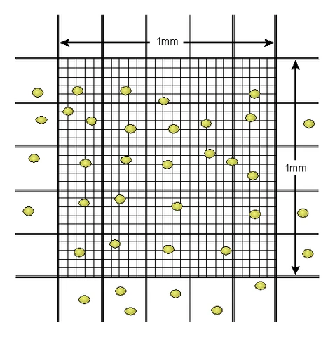A hemocytometer under the microscope. From https://di.uq.edu.au/community-and-alumni/sparq-ed/sparq-ed-services/using-haemocytometer

Here’s the idea in more detail, (quoted from my sister blog, DataOrigami.net):

The hemocytometer is designed such that a known quantity of volume exists under the inner 25 squares (usually 0.0001 mL). The observer will apriori pick 5 squares to count cells in, typically the 4 corner squares and the middle square. (Why only 5? Unlike this image above, there could be thousands of cells, and counting all 25 squares would take too long). Since we know the volume of the 25 squares, and the dilution rate, we can recover our original slurry concentration:

$$\text{cells/mL}=(\text{cells counted})⋅5⋅(\text{dilution factor})/0.0001\text{mL}$$

Given I counted 49 cells and my dilution was three 10x, my estimate is 2.45B cells/mL. Great! We are done, right? No way, consider all the sources of uncertainty we glossed over:

• Did we accurately measure out exactly 9mL of water in each test tube during dilution?
• Did we accurately extract 1mL of culture between each test tube?
• Did we get lucky/unlucky with our 0.0001 mL sample for the hemocytometer?
• Did the hemocytometer manufacturer have some QA over the volume of the chamber?
• Did we get lucky/unlucky with cells numbers in the 5 counting squares?

So we should expect high variance in our estimate because of the many sources of noise, and because the noises are layered on top of one another (i.e. a measurement error in one step is propagated down).

In the article on DataOrigami.net, I’ve coded up a Bayesian model to account for all these uncertainties, and thus produce an estimate of cell density and a better measure of uncertainty in that estimate. Returning to my example, if I counted 49 cells after three 10x serial dilutions, my estimate of cell density is 2.25B cells/mL with 95% credible intervals (1.76B cells/mL, 2.78B cells/mL).

Great, now that I’ve have an accurate cell density estimate and its uncertainty with hemocytometers, I can move on and say: I hate hemocytometers. Sigh. They require dilutions which are messy, they require manually counting to hundreds, they require me to keep some state in my head of “have I counted this cell yet?” - they just aren’t pleasant to work with. I’d like a faster method, with maybe less accuracy, but still a measure of uncertainty.

Secchi stick

A Secchi stick is a long ruler with a target on one end that is placed in a solution. The Secchi stick is lowered until the target at the end can’t be seen anymore, at which point we measure how far down we’ve lowered the stick. The principle behind this technique is that higher cell concentration causes less visibility in the solution (the technical term for this is turbidity). See figure 2 for a Secchi stick in action.

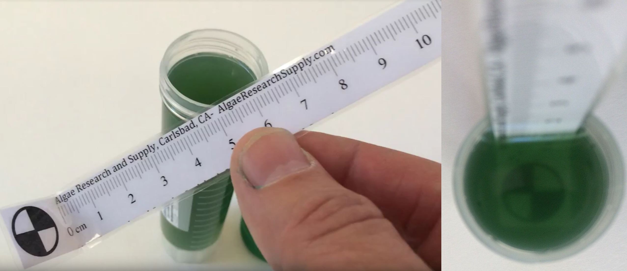Figure 2. A Secchi stick measuring algae. From https://algaeresearchsupply.com/

A Secchi stick provides a quick way to measure turbidity, and hence is correlated to cell density, but I’m missing an explicit connection. For example, if my Secchi stick measures 1.5cm, what cell density does that correspond to? The idea of correlating an efficient measurement with a more accurate, but more costly, measurement is common in industry and the sciences. So long as that correlation is valid and robust, we can replace the costly measurement with the efficient one. We call this a correlation model. How might we do this?

We first need to collect some data between the two measurements. In the past few weeks, while I’ve been growing my Nanno algae, I have taken the time to perform both a Secchi depth measurement and a hemocytometer measurement. Below is the raw data:

Secchi depth (cm)	hemocytometer count
1.4	310
2.4	148
1.7	241

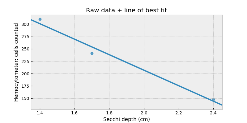
We could just naively plot this with a line-of-best-fit:

$$\text{cell count} = \alpha \cdot \text{depth} + c $$

However, look what happens when we try to extrapolate to depths beyond 3.5cm:

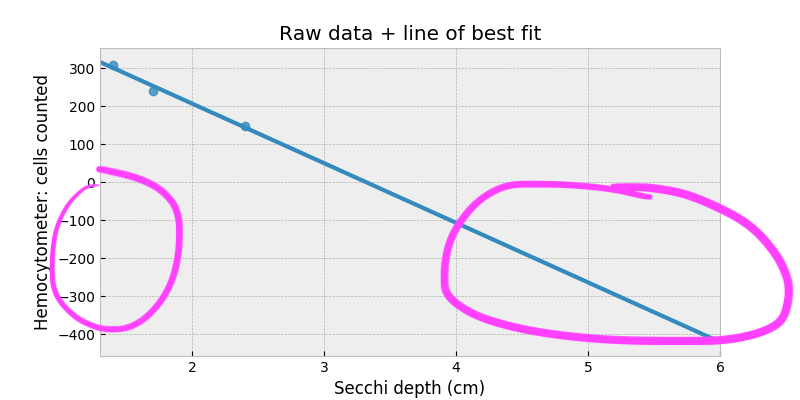
Our correlation model suggests we should start to see negative cell counts! Clearly something is wrong. We’ll fix this by considering a thought experiment: suppose there are no cells in the culture. How far down should the Secchi depth be? Assuming crystal clear water (which is fine considering our range of depths), we should have Secchi depth equal infinity! This relationship suggests we should be modeling with a logarithm somewhere. Something like:

$$\log{\text{cell count}} = \alpha \cdot \text{depth} + c $$

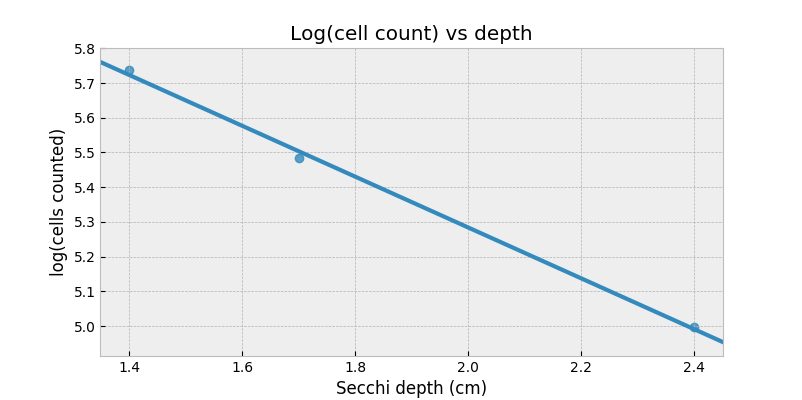
Now, the right-hand-side can be negative and that’s totally okay: a negative logarithm is just a value between 0 and 1.

Up until now, we’ve been considering modeling the cell count, but we are actually interested in the cell density. We could use our model above to predict a cell count, and then plug this into our Bayesian cell density model above. But, I consider this silly. The problem is any uncertainty in our prediction model (and remember we only have three data points) can’t be easily added to our cell density model. We should instead model this as one larger model. Going a step further, we really should be modeling the direct relationship between cell density and Secchi depth, without having to think about cell counts.

$$\log{\text{cell/mL}} = \alpha \cdot \text{depth} + c $$

Our new model looks like (ignoring dilutions):

$$ \begin{align} & \text{cell/mL} \sim \text{LogNormal}(\mu=\alpha \cdot \text{depth} + c, \tau) \\ & \;\;\;\; \alpha \sim \text{Normal}(0, 10) \\ & \;\;\;\; c \sim \text{Normal}(0, 10) \\ & \;\;\;\; \tau \sim \text{Exponential}(0.1) \\ & \text{cells in visible portion} \sim \text{Poisson}(\text{cell/mL} \cdot \text{volume of chamber}) \\ & \;\;\;\; \text{volume of chamber} \sim \text{Normal}(10^{-4}, 8\cdot10^{-6}) \\ & \text{cell count} \sim \text{Binomial}(N=\text{cells in visible portion}, p=5/25) \end{align} $$

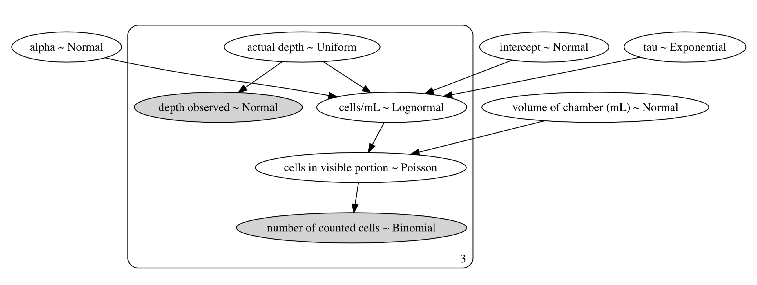
The way this model is presented above may be difficult to read, so here’s a directed-acyclic-graph (DAG) of our model:

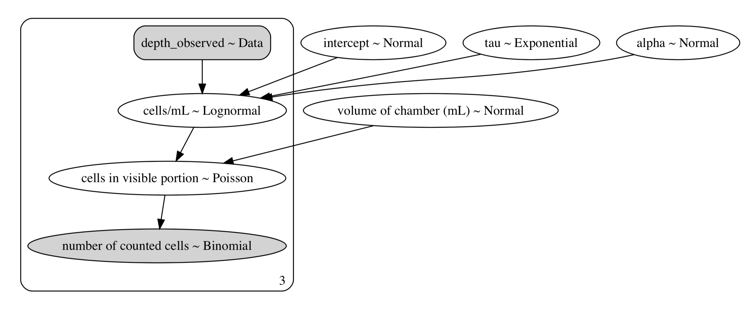DAG of our Secchi - hemocytometer correlation model. Dark areas are observed data, and light areas are random variables

And here’s the Python code to run our Bayesian model:

import pymc3 as pm

BILLION = 1e9
TOTAL_SQUARES = 25

squares_counted = 5
cells_counted = np.array([310, 148, 241])
depth_observed = np.array([1.4, 2.4, 1.7])
N = cells_counted.shape[0]

with pm.Model() as model:
    alpha = pm.Normal("alpha", mu=0, sd=10)

    # I need a test value here because of under/over flow problems.
    intercept = pm.Normal("intercept", mu=0, sd=10, testval=15)
    tau = pm.Exponential("tau", 0.1)

    cells_conc = pm.Lognormal("cells/mL", mu=alpha * depth_observed + intercept, tau=tau, shape=N)

    final_dilution_factor = 1
    # the manufacturer suggests that depth of the chamber is 0.01cm ± 0.0004cm. Let's assume the worst and double the error.
    # the length of the 5x5 square grid is 1mm = 0.1cm, so the volume is 0.01 * 0.1 * 0.1 = 0.0001, with error 0.1 * 0.1 * 0.0004 * 2
    volume_of_chamber = pm.Normal("volume of chamber (mL)", mu=1e-4, sd=8e-6)

    # why is Poisson justified? in my final shaker, I have cells_conc * final_dilution_factor * shaker3_volume number of cells
    # I remove volume_of_chamber / shaker3_volume fraction of them, hence it's a binomial with very high count, and very low probability.
    cells_visible = pm.Poisson("cells in visible portion", mu=cells_conc * final_dilution_factor * volume_of_chamber, shape=N)

    number_of_counted_cells1 = pm.Binomial("number of counted cells", cells_visible, squares_counted/TOTAL_SQUARES, observed=cells_counted)


    trace = pm.sample(18000, tune=14000)

After running it, we can inspect our quantities of interest: alpha and intercept (the latter is what we call c above):

pm.plot_posterior(trace, var_names=["alpha", "intercept"])

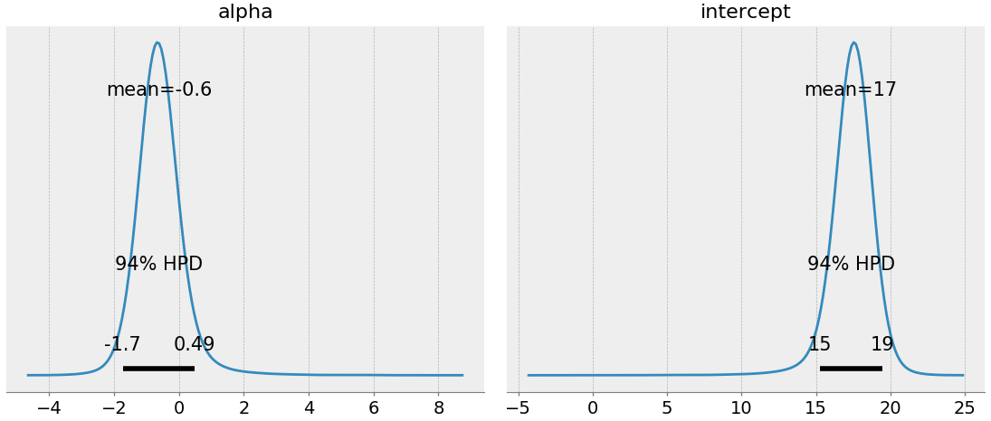
To explain this: we suspect alpha is around -0.6 (which makes sense, since depth should have a negative correlation with cell density), and the intercept is around 17. Naively, we could write down our correlation model as:

$$\log{\text{cell/mL}} = -.63 \cdot \text{depth} + 17.3 $$

This is okay, but it ignores all the uncertainty we just spent time modeling: recall we only have three data points, and our cell/mL is a noisy estimate. Instead, we can plot our 90% credible intervals along with our cell density prediction (top figure is in log-space):

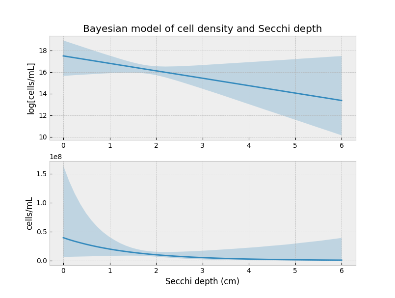
Notice how the uncertainty decreases around our three observations. This isn’t a coincidence. We have the most information about what the curve looks like here. Everything outside this domain is extrapolation.

How good are your eyes, though?

There’s one more piece of uncertainty we should be modeling. There is certainly some measurement error when I read the Secchi depth. This could be because of different light conditions, or an unsteady hand, or some warping due to water level. Either way, we can model this measurement error in our model. We append our model with the following:

$$ \begin{align} & \text{cell/mL} \sim \text{LogNormal}(\mu=\alpha \cdot \text{actual depth} + c, \tau) \\ & \;\;\;\; \text{actual depth} \sim \text{Uniform}(0, 10)\\ & \;\;\;\; \;\;\;\; \text{observed depth} \sim \text{Normal}(\text{actual depth}, 0.1)\\ & \dots \\ \end{align} $$

In the above, I’m saying that my measurement error is probably ±0.1 the actual value (whatever that means). Rerunning the model (code here) and reproducing the above figure:

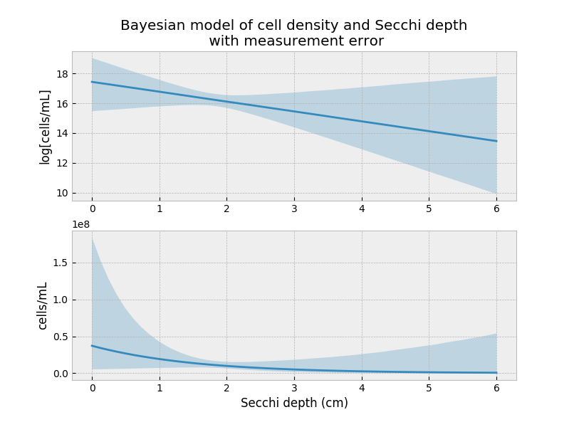
The predictions are not that different from the first model, but that could be due to the small measurement error that I introduced.

Conclusion

This is great: I can dip my Secchi stick into my algae and get a good estimate of the cell density, without having to perform a hemocytometer count. However, because different cell species will have different turbidity, I can only use this inference for my Nanno cultures (where the original data came from). I hope now the image below makes sense!